I have spent a lot of time working with distributed systems, and one challenge consistently stands out: managing unbounded data streams. Whether you are dealing with smart cities, healthcare sensors, or V2X communications, the data workloads often fluctuate dynamically and unpredictably.
In practice, I noticed engineers were constantly forced into a frustrating, manual compromise. When relying on static configurations, you either over-provision your resources and burn through your infrastructure budget, or you under-provision and watch your pipeline choke under backpressure.
That is exactly why I built Streamline. I wanted to build a multi-layer auto-tuning framework that doesn’t just react to problems, but anticipates them.
Quick Start & Installation
Getting Streamline running locally or on your cluster is straightforward.
1 | # Clone repository |
You can test the implementation using the provided examples in the /examples directory:
1 | # Run an example of a single data pipeline |
Step-by-Step: How Streamline Works
Step 1: Model Training
Before touching any live application, Streamline trains its underlying machine learning models. It pre-trains a Time Series Transformer (for workload prediction), a Neural Network (as a surrogate to estimate Apache Flink performance), and a Polynomial Regression model (to map max processing limits).
1 | INFO: Starting Workload Predictor training using Transformers... |
Step 2: Proactive Prediction & Auto-Tuning
When a new application is submitted, Streamline predicts the incoming workload for the source operators using the Transformer model, and calculates downstream loads using historical aspect ratios.
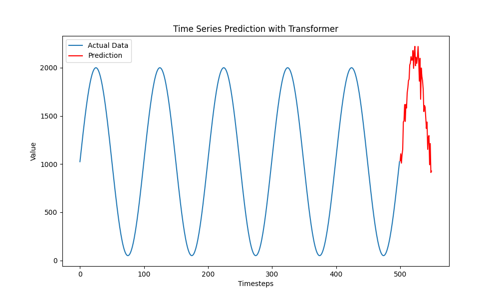
It then feeds these predictions into an NSGA-II evolutionary algorithm. Using the Neural Network as a surrogate evaluator, it finds optimized configuration parameters (parallelism and buffer-size) and estimates cpu, end-to-end-latency, and throughput for each operator.
1 | INFO: Predicting workload of operators using Transformers and aspect ratio... |
Step 3: Resource-Aware Scheduling
With the configurations set, the scheduler dynamically maps the operator instances to your available compute resources (TaskManagers).
1 | INFO: Total required CPU: 5.703662050962448 |
Step 4: Periodic Re-evaluation (Dynamic Adaptation)
Streamline runs at regular intervals to verify if the applications need updates based on shifting data streams. For instance, if the workload of the application drops, Streamline automatically scales down its parallelism (from 4.0 to 2.0) to save resources, while leaving other applications untouched.
Evaluation
Streamline was evaluated on the Grid 5000 testbed using real-world IoT and streaming benchmarks.
| Metric | Maximum Improvement |
|---|---|
| End-to-end Latency | 10x |
| Monetary Costs | 10x |
| CPU Utilization | 9x |
| Throughput | 4x |
If you are dealing with large-scale, volatile data stream applications, or are interested in a more in depth description of Streamline or its evaluation results, I encourage you to read the full paper or explore the Streamline repository on GitHub.